MathMap is a GIMP plug-in that allows moderately sophisticated users to describe image transforms and combinations using a straightforward language. MathMap even builds a user interface for the parameters to your expression, so it is an ideal system for prototyping many types of image processing operations.
Because MathMap operates on a per-pixel basis and compiles expressions with your C compiler, it is fast enough to explore new fractal renderings. Coupled with access to The GIMP's gradients, curves, and other images, MathMap can create images that would be impossible with programs like the venerable Fractint.
I will give a brief introduction to Mandelbrot-style fractals and then throw a whole bunch of assumptions out the door and show you how to make some totally crazy images and animations in MathMap.
This paper is about two things - MathMap and fractals. I'll give a very brief introduction of MathMap, then proceed to show how it can be used for rapid prototyping of image processing and rendering effects, in particular, fractals.
All of this is a work in progress, so many as-yet-unimplemented ideas will be discussed, and the provided code examples may have bugs -- they certainly have inconsistencies.
This is impure mathematics. Any mathematical notation that has crept into this paper is a result of the convenience of the notation and does not indicate any strict mathematical rigour or definiton.
I am a great fan of mathematics, so naturally a plug-in with the name MathMap caught my eye. MathMap is a GIMP plug-in that allows moderately sophisticated users to describe image processing algorithms in a very expressive pixel-focussed language. If an algorithm can be summarized as a function that takes an x,y (or r,a) coordinate and (optionally) a single time t parameter, then it can probably be implemented in MathMap.
MathMap constructs a GTK+ user interface summarizing all parameters to your function. It compiles your code fairly efficiently with gcc, so it is an ideal system for prototyping many types of image processing operation.
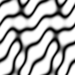
For example, the GIMP plug-in 'Displace' displaces pixels in an image based on offsets in two grayscale images - one for displacement in X, and one for displacement in Y. Here's a MathMap expression which does the same thing in polar coordinates:
    origVal(ra:[r + t*user_slider("MaxR",0,32)
                  * ((2*gray(origVal(xy,user_image("Radial"))))-1),
                a + t*user_slider("MaxA",0,360)
                  * ((2*gray(origVal(xy,user_image("Angle"))))-1)])
A brief explanation:
With MathMap's built-in antialiasing facilities [1], this expression provides an excellent "Radial Displace" function. In fact, many simple GIMP plug-ins could be reimplemented in MathMap.
You can learn more about MathMap at http://www.complang.tuwien.ac.at/~schani/mathmap/ .
Fractals are a very widely explored field these days, so I'm not going to go into the history or all the different types of fractals out there. Please just check Google for more information: http://www.google.com/search?q=fractals .
When it comes down to it, fractals are patterns that emerge upon the iteration certain mathematical/geometrical operations. These patterns are often beautiful and strange and terrifying. The MathMap expressions in this paper render Mandelbrot-style fractals with a few image-based twists thrown in.
The Mandelbrot set is, briefly, the set of all complex numbers c which, when you start with z=0+0i and iterate z=z2+c, the magnitude of z doesn't go off to infinity. Of course z goes to infinity quite quickly after |z| reaches 2, so we just check that |z|<2. After some number of interations, we give up and assume that a point is in the set. Since we like pretty things, we colour the escaping pixels (those not in the set) according to how many iterations we went through before they escaped. There are also interesting ways to colour pixels that are in the set, but this paper does not cover them.
Here's an expression which is distributed with MathMap, to visualize the Mandelbrot set. It goes through at most 31 iterations and colours pixels using the current GIMP gradient. [2]
    c=ri:(xy/xy:[X,X]*1.5-xy:[0.5,0]);
    z=ri:[0,0];
    iter=0;
    while
        abs(z)<2 && iter<31
    do
        z=z*z+c;
        iter=iter+1
    end;
    gradient(iter/32)
We can make an animation of this image that cycles the colours by replacing the final line with something like:
gradient(((iter/8)+t)%1.0)
The escape criterion for our simple Mandelbrot set was |z|>2. Let's think of this another way. What if we take the complex plane and colour the outside of the 2-unit circle with white and the inside with black, and after each iteration we add the colour value (where white=1.0 and black=0.0) at z to an accumulator. When that accumulator reaches 1.0, we say that we have 'escaped'. This is equivalent to |z|>2. We have replaced the escape function with an escape accumulator.
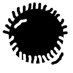
Of course, we've now assumed that this accumulation map is just an abstract object in the plane. Instead, let's represent it as a grayscale image and draw on it in the GIMP and see what happens. Of course we're going to end up with aliasing when we draw a circle on a rectangular grid. However, the image no longer has to be strictly black & white and there's no reason that it has to be a regular geometric shape.
This process is called the Xach Transform after #gimp denizen and Phlux groupie Zachary Beane.
All of the expressions are in examples.txt and all of the GIMP XCF files produced with them are in examples-xcf.tar.gz.
The first and simplest example uses this MathMap expression:
    bailout = user_slider("bailout", 1, 64);
    maxiter = user_slider("max.iter", 64, 2048);

    mesc = user_image ("accumulation_map");

    mxmin = user_slider("Map_X_Min", -5, 5);
    mxmax = user_slider("Map_X_Max", -5, 5);
    mymin = user_slider("Map_Y_Min", -5, 5);
    mymax = user_slider("Map_Y_Max", -5, 5);

    c = ri:[lerp(x/X, user_slider("Img_X_Min", -0.5, 1.0),
                      user_slider("Img_X_Max", -0.5, 1.0)),
            lerp(y/Y, user_slider("Img_Y_Min", -0.75, 0.75),
                      user_slider("Img_Y_Max", -0.75, 0.75)) + 0.75];

    scalex = X / (mxmax - mxmin);
    scaley = Y / (mymax - mymin);

    z = c;
    accum = 0;
    iter = 0;

    while ((accum < bailout) && (iter < maxiter)) do
        z = (z^2) + c;
        accum = accum + gray(origVal(xy:[scalex * z[0], scaley * z[1]], mesc));
        iter = iter + 1;
    end;

    gradient (((iter/maxiter)^0.2)%1.0)
Briefly, the parameters are:
With this input image as the accumulation map (and the appropriate parameters), we get an image in which the effects of the squiggles drawn on the circle are visible in the resulting image (a bit of sharpening was applied to make them more visible):


To make these effects even more visible, we can progressively rotate the accumulation map. Note that we're using some more sophisticated mathematics and MathMap functions:
    c = ri:[lerp(x/X, user_slider("T_min_X", -0.5, 1.0),
                     -user_slider("T_max_X", -1.0, 0.5)),
            lerp(y/Y, user_slider("T_min_Y", -0.75, 0.75),
                     -user_slider("T_max_Y", -0.75, 0.75))+0.75];

    minx = user_slider("M_min_X", -5, 5);
    maxx = -user_slider("M_max_X", -5, 5);
    miny = user_slider("M_min_Y", -5, 5);
    maxy = -user_slider("M_max_Y", -5, 5);

    threshold = user_slider("Threshold", 1, 64);
    maxcount = user_slider("Max.Iter", 64, 2048);

    xscale = X / (maxx - minx);
    yscale = Y / (maxy - miny);

    z = ri:[0,0];

    accum = 0;
    count = 0;

    ang = 360 * t;
    rmat = m2x2:[cos(ang), -sin(ang), sin(ang), cos(ang)];

    while ((accum < threshold) && (count < maxcount)) do
        z=(z^2) + c;
        accum = accum + gray(origVal((xy:[xscale * z[0],
                                          yscale * z[1]]) * rmat,
                             user_image("Accumulation Map")));
        count = count + 1;
    end;

    gradient ((16*count/maxcount)%1.0)
A few of the parameters were renamed here, and I changed the sign of the _max_ coordinates so I wouldn't have to keep pulling those sliders over to the right. Here are the results:


The iteration function for our simple Mandelbrot set was z=z2+c. Even in the simplest of cases, this function reveals beautiful and mysterious images. Of course we can use other powers or other functions, but if you've been paying attention, you'll know that this paper is about using images as parameters to fractal functions. So, the next experiment was to alter the value of z after each iteration, based on the value of a user-specified image.
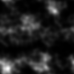
How about if we nudge z a little bit after each iteration based on the image value? In this example, we use a solid noise function to alter the radius of z at each iteration. We animate the image by rotating the map as before.
    c = ri:[lerp(x/X, user_slider("T_min_X", -0.5, 1.0),
                     -user_slider("T_max_X", -1.0, 0.5)),
            lerp(y/Y, user_slider("T_min_Y", -0.75, 0.75),
                     -user_slider("T_max_Y", -0.75, 0.75))+0.75];

    minx = user_slider("M_min_X", -2, 2);
    maxx = -user_slider("M_max_X", -2, 2);
    miny = user_slider("M_min_Y", -2, 2);
    maxy = -user_slider("M_max_Y", -2, 2);

    threshold = user_slider("Threshold", 2, 64);
    maxcount = user_slider("Max.Iter", 64, 2048);

    xscale = X / (maxx - minx);
    yscale = Y / (maxy - miny);

    z = ri:[0,0];

    accum = 0;
    count = 0;

    ang = 360 * t;
    rmat = m2x2:[cos(ang), -sin(ang), sin(ang), cos(ang)];

    while ((abs(z) < threshold) && (count < maxcount)) do
        z = (z^2) + c;
        z = z * (gray(origVal((xy:[xscale * z[0], yscale * z[1]])*rmat))
                 + user_slider("mult_offset",0.5,1));
        count = count + 1;
    end;

    gradient (((4*count/maxcount)%1.0)^0.25)
In this expression, the mult_offset parameter is used to shift the 0.0 - 1.0 range of the radius multiplier. As always, the exact parameters are left as an exercise for the reader -- here are my first results:


I must admit that I was surprised by that one ... wow.
Here's another nifty one: we alter the power to which z is raised at each iteration based on the image value.
    c = ri:[lerp(x/X, user_slider("T_min_X", -0.5, 1.0),
                     -user_slider("T_max_X", -1.0, 0.5)),
            lerp(y/Y, user_slider("T_min_Y", -0.75, 0.75),
                     -user_slider("T_max_Y", -0.75, 0.75))+0.75];

    minx = user_slider("M_min_X", -4, 4);
    maxx = -user_slider("M_max_X", -4, 4);
    miny = user_slider("M_min_Y", -4, 4);
    maxy = -user_slider("M_max_Y", -4, 4);

    threshold = user_slider("Threshold", 2, 64);
    maxcount = user_slider("Max.Iter", 64, 2048);

    xscale = X / (maxx - minx);
    yscale = Y / (maxy - miny);

    z = ri:[0,0];

    accum = 0;
    count = 0;

    ang = 360 * t;
    rmat = m2x2:[cos(ang), -sin(ang), sin(ang), cos(ang)];

    while ((abs(z) < threshold) && (count < maxcount)) do
        pow = gray(origVal((xy:[xscale * z[0], yscale * z[1]])*rmat))
                 + user_slider("Power Offset",0.5,2);
        z = (z^pow) + c;
        count = count + 1;
    end;

    gradient (((4*count/maxcount)%1.0)^0.25)
The "Power Offset" parameter shifts that 0.0 - 1.0 range around as usual. Of course using the lerp() function would be more general but if I did everything that popped into my head I'd never get anything else done.


The thing I love about this stuff is that I never know what to expect. This image freaked me out so much that I declined to animate it.
Another way to nudge z it to make a height field and move it along the slope at each point. I chose to animate this by estimating the X and Y slope at each pixel using the bumpmap plugin, then weighting the X and Y slope factor with a point moving around a circle.
    bailout = user_slider("bailout", 2, 64);
    maxiter = user_slider("max.iter", 64, 2048);

    xgrad = user_image("x_gradient");
    ygrad = user_image("y_gradient");
    gslope = 2*user_slider("gradient_slope", 0, 8);
    ang = t*360;
    cosang = cos(ang);
    sinang = sin(ang);
    gsx = cosang*gslope;
    gsy = sinang*gslope;
    rmat = m2x2:[cosang, -sinang, sinang, cosang];

    mxmin = user_slider("map_x_min", -2, 2);
    mxmax = -user_slider("map_x_max", -2, 2);
    mymin = user_slider("map_y_min", -2, 2);
    mymax = -user_slider("map_y_max", -2, 2);

    c = ri:[lerp(x/X, user_slider("img_x_min", -0.5, 1.0),
                     -user_slider("img_x_max", -1.0, 0.5)),
            lerp(y/Y, user_slider("img_y_min", -0.75, 0.75),
                     -user_slider("img_y_max", -0.75, 0.75)) + 0.75];

    scalex = X / (mxmax - mxmin);
    scaley = Y / (mymax - mymin);

    z = c;
    iter = 0.0;

    while (abs(z) < bailout && (iter < maxiter)) do
        z = (z*z) + c;
        zp = xy:[scalex * z[0], scaley * z[1]];
        z = ri:[z[0] + gsx*(gray(origVal(zp, xgrad)-0.5)),
                z[1] + gsy*(gray(origVal(zp, ygrad)-0.5))];
        iter = iter + 1;
    end;

    if (iter == maxiter) then
        rgba:[0,0,0,1];
    else
        gradient ((16*iter/maxiter+t)%1.0);
    end


MathMap allows multiple user-specified images, so any of the above techniques can be combined. Here's an animation with colour cycling, an accumulation map, a power-changing map, and a radius-changing map:
    maxiter = user_slider("Maximum Iterations", 64, 2048);
    bailout = user_slider("Accumulation Bailout", 2, 64);
    mesc = user_image("Accumulation Map");

    mpow = user_image("Power Map");
    opow = user_slider("Power Offset", 0.5, 2.0);

    mrad = user_image("Radius Map");
    orad = user_slider("Radius Offset", 0.5, 1.0);

    mxmin = user_slider("Map X Min", -5, 5);
    mxmax = -user_slider("Map X Max", -5, 5);
    mymin = user_slider("Map Y Min", -5, 5);
    mymax = -user_slider("Map Y Max", -5, 5);

    scalex = X / (mxmax - mxmin);
    scaley = Y / (mymax - mymin);

    c = ri:[lerp(x/X, user_slider("Img X Min", -0.5, 1.0),
                      -user_slider("Img X Max", -0.5, 1.0)),
            lerp(y/Y, user_slider("Img Y Min", -0.75, 0.75),
                      -user_slider("Img Y Max", -0.75, 0.75)) + 0.75];

    ang = t*360;
    rmat = m2x2:[cos(ang), -sin(ang), sin(ang), cos(ang)];

    z = c;
    iter = 0.0;
    accum = 0.0;

    while ((accum < bailout) && (iter < maxiter)) do
        pow = gray(origVal((xy:[scalex * z[0], scaley * z[1]])*rmat, mpow)) + opow;
        z = (z^pow) + c;
        zp = xy:[scalex * z[0], scaley * z[1]] * rmat;
        z = z * (gray(origVal(zp, mrad)) + orad);
        accum = accum + gray(origVal(zp, mesc));
        iter = iter + 1;
    end;

    if (iter == maxiter) then
        rgba:[0,0,0,1];
    else
        gradient((((32*iter/maxiter)^0.5) + t)%1.0);
    end


That took over 16 hours to render but I think it was worth the wait.
The examples presented so far are the tip of the iceberg. Essentially anything can be done to z at each iteration, and MathMap makes it easy to look up per-pixel values as additional arguments.
All of the input map images described in this paper have been grayscale; more could be done in the RGB or HSV colourspaces. For example, three grayscale images (e.g. the RGB channels of an image) could be used as accumulation maps for the corresponding channel in the output image. This would of course take 3 times as long to calculate but might look interesting.
I have chosen to animate these images by rotating the maps used during calculation. It might be interesting to replace a map with a video stream or other free-form animation, such as an animated distortion as produced by the GIMP IWarp plugin.
This has been a brief tour of the possibilities of using the MathMap plug-in to render Mandelbrot-style fractals, distorted by images. Welcome to the world of impure mathematics.
1 MathMap's antialiasing facilites are really nice, but well outside the scope of this paper.
2 I modified this expression to use my z and c terms because I've been doing this stuff for over 10 years and I know them as z and c.
© Copyright June 2001 by
Tom Rathborne -
tomr@aceldama.com
This document, the ideas it reveals, and its associated images are in the public domain.